The series solution of second-order linear differential equations with variable coefficients explores the general form of such equations, detailing their applications in engineering, particularly in mechanical and electrical vibrations. This document provides a comprehensive overview of homogeneous and non-homogeneous equations, including methods for finding complementary functions and particular integrals. Key examples illustrate the solution process for various equations, making it a valuable resource for students and professionals in mathematics and engineering fields. The content is particularly useful for those studying differential equations and their applications in real-world scenarios.

Key Points

  • Explains the general form of second-order linear differential equations with variable coefficients.
  • Covers methods for solving homogeneous and non-homogeneous equations.
  • Includes examples demonstrating the solution process for various differential equations.
  • Discusses applications in engineering, particularly in mechanical and electrical vibrations.
Ekemini Tom
14 pages
Language:English
Type:Solution Manual
Ekemini Tom
14 pages
Language:English
Type:Solution Manual
331
/ 14
1
SERIES SOLUTION OF SECOND ORDER LINEAR DIFFERENTIAL EQUATIONS
WITH VARIABLE COEFFICIENTS
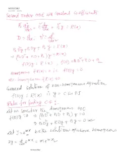
The second-order linear differential equations with variable coefficients are differential
equations whose coefficients are a function of a certain variable. A second-order linear
differential equation has a general form



󰆒󰆒
󰆒
󰇛󰇜
where P, Q, R and G are functions of the independent variable x. If P, Q and R are some constant
quantities, then the above equation is known as a second-order linear differential equation with
constant coefficients. If G = 0 then the equation is called a homogeneous linear differential
equation of second order, otherwise it is non-homogenous.
A second-order ODE is called linear if it can be written in the form in Eqn. (1) above and
nonlinear if it cannot be written in this form.
These equations have important engineering applications, especially in connection with
mechanical and electrical vibrations, as well as in wave motion, heat conduction, and other
parts of physics
Solutions to Homogeneous 2
nd
Order DE
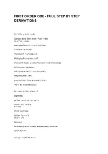
Solution of a second order differential equation consisting of two parts; a complementary
function which is the solution of the differential equation whose R.H.S. is zero and a particular
integral which relates the RHS to the LHS of the equation
Thus, Complete Solution = Complementary Function + Particular Integral
 
To solve a second order homogeneous ODE when G(x) = 0, we look at the characteristic
equation, obtained by replacing the differentials in the form
 
The solution to the quadratic equation above gives a three-case solution: the case when the
roots of the characteristic equation are distinct and real, complex or equal.
CASE I: When
 The Roots are Real and Different





CASE II: When
 The Roots are Real and Equal




󰇛 󰇜
CASE III: When
 The Roots are complex





󰇛󰇜
Examples
1. Solve the equation
󰆒󰆒
󰆒

Solution
󰇛
󰇜󰇛
󰇜




2. Solve the equation 
󰆒󰆒

󰆒

Solution


󰇛

󰇜󰇛

󰇜
󰇛 󰇜
3. Solve the equation
󰆒󰆒

󰆒

Solution
2
 


 
󰇛󰇜
󰇛󰇜󰇛󰇜
󰇛󰇜
 󰇛󰇜󰇛󰇜
󰇛󰇜
 




󰇛 󰇜
4. Solve the equation
󰆒󰆒

󰆒

5. Solve the equation
󰆒󰆒

󰆒

6. Solve the equation
󰆒󰆒

󰆒

Initial value or boundary problems
1. Solve the equation
󰆒󰆒
󰆒

󰇛
󰇜

󰆒
󰇛
󰇜
Solution
󰇛
󰇜󰇛
󰇜




󰇛
󰇜

󰇛󰇜
󰆒
󰇛
󰇜






 󰇛󰇜

󰇛
󰇜
 󰇛󰇜

󰇛
󰇜
󰇛
󰇜
 

󰇛
󰇜
The required solution of the initial-value problem is


2. Solve the boundary-value problem
󰆒󰆒

󰆒
󰇛
󰇜

󰇛
󰇜

󰇛
󰇜󰇛
󰇜





󰇛
󰇜


󰇛󰇜
󰇛
󰇜



󰇛󰇜
Thus,


󰇛󰇜
Multiplying equation 3 by e

So that
 
Giving the solution

󰇛 󰇜

3. Solve the boundary-value problem
󰆒󰆒

󰇛
󰇜

󰇛

󰇜
4. Solve the boundary-value problem
󰆒󰆒

󰆒

󰇛
󰇜

󰇛
󰇜
5. Solve the boundary-value problem
󰆒󰆒

󰆒

󰇛
󰇜

󰇛
󰇜

6. Solve the boundary-value problem
󰆒󰆒

󰆒

󰇛
󰇜

󰆒
󰇛
󰇜
7. Solve the initial – value problem
󰆒󰆒

󰇛
󰇜

󰆒
󰇛
󰇜

3
Operator D solution to ODE
Differential operator: Symbol D stands for the operation of differential i.e.,



And


Thus,



Can be written as
󰇛


󰇜
RULES TO FIND PARTICULAR INTEGRAL
󰇛
󰇜
󰇛
󰇜

󰇛
󰇜


󰇛
󰇜

󰇛
󰇜

󰆒
󰇛
󰇜


󰆒
󰇛
󰇜

󰇛
󰇜

󰆒󰆒
󰇛
󰇜

󰇛

󰇜
󰇛󰇜
󰇟󰇛󰇜󰇠

󰇛

󰇜
󰇛
󰇜

󰇛

󰇜

󰇛
󰇜

󰇛

󰇜


󰇛

󰇜

󰇛
󰇜

󰆒
󰇛
󰇜

󰇛

󰇜
󰇛
󰇜

󰇛
󰇜

󰇛
󰇜

󰇛
󰇜
󰇛
󰇜
󰇛
󰇜


󰇛
󰇜

Examples
1. Solve the equation




Solution


󰇛
󰇜󰇛
󰇜
󰇛󰇜





󰇛 󰇜


󰇛

󰇜




󰇛

󰇜


Applying
󰇛
󰇜

󰇛
󰇜


We have
󰇛
󰇛󰇜
󰇜






So, the complete solution is:


󰇛

󰇜




/ 14
End of Document
331

FAQs

What is the general form of a second-order linear differential equation with variable coefficients?
The general form of a second-order linear differential equation with variable coefficients is given by P(d²y/dx²) + Q(dy/dx) + Ry = G, where P, Q, R, and G are functions of the independent variable x. If P, Q, and R are constant quantities, the equation is classified as having constant coefficients. If G equals zero, it is referred to as a homogeneous linear differential equation; otherwise, it is non-homogeneous.
How do you find the complementary function of a homogeneous second-order ODE?
To find the complementary function of a homogeneous second-order ordinary differential equation (ODE), one must solve the characteristic equation obtained by replacing the differentials with a variable m. This leads to a quadratic equation of the form am² + bm + c = 0. Depending on the nature of the roots (real and distinct, real and equal, or complex), the complementary function can be expressed in different forms: for distinct roots, it is yCF = Ae^(m1x) + Be^(m2x); for equal roots, it is yCF = (A + Bx)e^(m1x); and for complex roots, it is yCF = e^(αx)(Acos(βx) + Bsin(βx)).
What are the three cases of roots in the characteristic equation?
The three cases of roots in the characteristic equation of a second-order linear differential equation are as follows: Case I occurs when the discriminant (b² - 4ac) is greater than zero, resulting in two distinct real roots. Case II occurs when the discriminant equals zero, leading to a repeated real root. Case III occurs when the discriminant is less than zero, resulting in complex roots. Each case leads to a different form of the complementary function in the solution of the differential equation.
What is the method to find a particular integral for non-homogeneous equations?
To find a particular integral for non-homogeneous second-order linear differential equations, one can employ the operator method. This involves expressing the equation in operator form, such as (PD² + QD + R)y = G. Specific rules apply based on the form of G, such as using the formula 1/f(D)e^(ax) = 1/f(a)e^(ax) if f(a) is not zero. If f(a) equals zero, further derivatives are used to find the appropriate particular integral.
What is the significance of the damping force in mechanical systems?
In mechanical systems, the damping force plays a crucial role in the behavior of oscillating systems, such as mass-spring systems. The damping force is proportional to the velocity of the mass and acts in the opposite direction to the motion. This leads to different damping scenarios: overdamping, critical damping, and underdamping, each characterized by the nature of the roots of the auxiliary equation. Understanding the damping force is essential for analyzing the stability and response of mechanical systems under various conditions.
How do initial value problems relate to second-order differential equations?
Initial value problems (IVPs) for second-order differential equations involve determining the solution of the equation given specific initial conditions, such as the value of the function and its derivative at a particular point. For example, solving the equation y'' + y' - 6y = 0 with initial conditions y(0) = 1 and y'(0) = 0 requires finding the complementary function and particular integral, then applying the initial conditions to solve for the constants involved in the general solution.
What are the applications of second-order linear differential equations?
Second-order linear differential equations have significant applications in various fields, particularly in engineering. They are used to model mechanical and electrical vibrations, wave motion, heat conduction, and other physical phenomena. Understanding these equations is crucial for analyzing systems in mechanical engineering, electrical circuits, and physics, as they describe how systems respond to forces and changes over time.