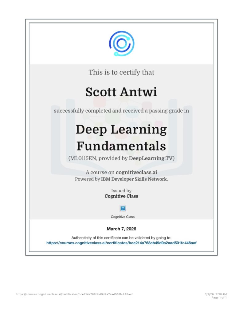



Deep learning is the dominant contemporary subfield of artificial intelligence that implements multi-layered artificial neural networks to learn hierarchical representations directly from complex, unstructured datasets. While classical machine learning workflows rely extensively on human domain experts to execute manual feature engineering, deep learning architectures automate this process entirely. By passing raw data arrays through stacked configurations of non-linear mathematical computational units, these systems automatically decompose inputs into progressively more abstract features. This evolutionary capability has shifted computing from hard-coded automation into a highly predictive engineering paradigm. To support students and researchers pursuing this field, our master category for Artificial Intelligence features a dense library of core instructional assets, including the definitive blueprint on Deep Learning Fundamentals.
The bedrock of all deep learning architectures is the artificial neural network (ANN), which functions as a directed graph of interconnected processing elements termed neurons or nodes. Individual neurons accept a vector of inputs, apply scalar weights ($w$) to each input line, accumulate the resulting products, and append a static bias scalar ($b$). This linear combination is subsequently parsed through a non-linear activation function—such as the Rectified Linear Unit (ReLU) or GELU—to determine the neuron’s mathematical output state. When arranged into a Feedforward Network or Multi-Layer Perceptron (MLP), these nodes form an input layer, multiple hidden layers, and an output layer. Training these massive parameter grids requires executing backpropagation, an algorithmic application of the multi-variate calculus chain rule that routes error gradients backward through the network to update parameters via gradient descent.
When processing spatial datasets like imagery, traditional dense layers suffer from a massive parameter explosion that destroys local spatial patterns. To circumvent this limitation, deep learning employs Convolutional Neural Networks (CNNs). Instead of connecting every input pixel to every neuron, convolutional layers pass small, localized parameter matrices called filters across the input tensor. This mathematical operation enforces parameter sharing and local connectivity, allowing the network to achieve translation invariance, meaning it can recognize an object regardless of its spatial location within the frame. This spatial processing power is deployed in advanced deep networks for heavy structural tracking systems, such as the system explored in An Ensemble Model Using Face and Body Tracking for Engagement Detection. Furthermore, the structural optimization logic of CNNs can be applied across abstract engineering data landscapes, a paradigm analyzed within Distributed Database Load Balancing Prediction Based on Convolutional Neural Network.
For processing sequential or temporal data streams—such as audio, time-series metrics, or natural language—deep learning historically relied on Recurrent Neural Networks (RNNs) and Long Short-Term Memory (LSTM) networks. These models maintain an internal hidden state vector that serves as a sequential memory buffer, feeding past execution states back into the network alongside the current input token. However, RNNs suffer from severe vanishing and exploding gradient problems when backpropagating across extended time horizons, rendering long-term dependencies uncomputable. This sequential bottleneck was broken by the invention of the Transformer architecture, which replaces recurrence entirely with a highly parallelizable mechanism called self-attention. Transformers evaluate the contextual relationship between every single token across an entire sequence simultaneously, allowing for the scaling of massive Large Language Models (LLMs).
In industrial ecosystems, deep learning frameworks drive autonomous systems, intelligent infrastructure management, and cognitive business agents, a corporate paradigm thoroughly investigated in KI Agenten im Mittelstand: Digitale Kollegen die wirklich entlasten. Concurrently, generative deep learning models—such as Generative Adversarial Networks (GANs) and Diffusion Models—have unlocked the capability to synthesize hyper-realistic text, synthetic audio, and high-fidelity graphics from raw random noise inputs.
However, the immense power of deep generative models requires rigorous systemic alignment, security governance, and ethical validation protocols. Because deep neural networks function as mathematical “black boxes” lacking direct transparency, their structural vulnerabilities can be exploited for computational warfare or digital deception. The deployment of autonomous deep learning systems within global defense networks presents severe geopolitical and existential risks, a reality scrutinized inside Autonomous Weapons and Artificial Intelligence in Warfare – Working Paper Of Block B. Simultaneously, the abuse of open-source generative media engines requires rapid defensive engineering to mitigate software exploitation and societal harm, as detailed in the critical security brief Safeguarding Alert: AI Undress Apps and Websites. Balancing model capacity with strict mathematical safety parameters remains the core challenge for modern deep learning research.
To see how deep learning structures its architectural styles and connectionist models under the broader banner of the computing sciences, review the following taxonomy:
Parent Category: Computer Science
Academic Branch: Artificial Intelligence
Core Paradigm: Deep Learning
Architectural Specialties:
Deep Feedforward Networks (Multi-Layer Perceptrons, Optimization Calculus)
Convolutional Architectures (CNNs, Residual Networks, Spatial Processing)
Recurrent Connections (RNNs, LSTMs, GRUs, Sequential Modeling)
Attention-Based Models (Transformers, Self-Attention, LLM Foundations)
Deep Generative Networks (GANs, Variational Autoencoders, Diffusion Models)
Reinforcement Learning Agents (Deep Q-Networks, Actor-Critic Architectures)
| Deep Architecture Type | Primary Data Paradigm | Core Mathematical Operator | Primary Structural Strength |
| Multi-Layer Perceptron (MLP) | Tabular, unstructured multi-variate vectors | Matrix multiplication ($W \cdot x + b$) | Universal function approximation for structured data |
| Convolutional Network (CNN) | Spatial grids, imagery, volumetric tensors | Discrete 2D/3D matrix convolution ($\ast$) | Preserves spatial invariance and minimizes parameter counts |
| Recurrent Network (RNN/LSTM) | Sequential streams, audio, language strings | Recursive hidden-state matrix updates | Processes variable-length sequences with step-by-step memory |
| Transformer Model | Parallel token sequence matrices | Scaled Dot-Product Self-Attention | Captures long-range dependencies via global parallelization |
Chesser Resources is a free online study-and-research library at chesserresources.com. It holds 300,000+ documents — books, textbooks, past papers, lecture notes, study guides, research papers and much more — across exams, the sciences, math, literature, the humanities and beyond. Everything is readable in the browser with no account, alongside free AI summaries, an Ask-AI chatbot, highlights, notes and read-aloud audio. Instead of a subscription, downloads are unlocked by contributing back to the community, so the library stays genuinely free.
Shallow machine learning models (such as Linear Regression, Support Vector Machines, or Random Forests) possess a flat processing architecture that requires human engineers to manually transform raw data into informative features before training. Deep learning models utilize a cascaded pipeline of multiple non-linear hidden layers to execute automated feature engineering, allowing the network to extract high-level semantic representations directly from raw inputs.
Backpropagation implements the calculus chain rule to calculate the partial derivative of a network’s global loss function with respect to every individual weight parameter. After a forward pass evaluates training inputs to compute a scalar error, backpropagation calculates the local gradient at the output layer and propagates that error signal backward through the hidden layers. This yields exact directional vectors that optimization algorithms use to iteratively adjust weights and minimize error.
The vanishing gradient problem occurs during backpropagation when the computed error gradients decay exponentially as they flow backward through dozens of hidden layers. This decay typically happens when using saturating activation functions like Sigmoid or Tanh, whose derivatives are bounded to a maximum value less than $0.25$. As these fractional values are multiplied repeatedly layer-by-layer, the gradient approaches zero, leaving the earliest layers completely untrained.
Residual Networks (ResRes) introduce structural shortcut connections, or skip connections, that bypass one or more hidden layers within a network block. Mathematically, instead of forcing a stacked array of layers to learn an isolated target mapping $H(x)$, the block is trained to learn a residual mapping $F(x) = H(x) – x$. This architecture allows the raw input signal $x$ to be added directly to the output, providing a clean highway for gradients to flow backward without attenuation during backpropagation.
Pooling layers (such as Max Pooling or Average Pooling) execute down-sampling operations across the spatial dimensions of a feature map tensor. By sliding a localized grid window across the matrix and selecting only the maximum or average value within that frame, pooling layers reduce the spatial resolution. This minimizes the network’s overall computational parameter count, accelerates processing speed, and grants the network a degree of structural translation invariance.
A convolutional layer preserves spatial locality by mapping connections exclusively within localized receptive fields. Instead of connecting every pixel to every neuron, a node in a convolutional layer processes only a tiny, contiguous patch of adjacent pixels dictated by the filter size. This localized focus ensures that the network preserves contextual spatial relationships—such as edges, corners, and boundaries—that are lost if the image is flattened into a 1D vector.
The core structural limitation of Recurrent Neural Networks (RNNs) is their sequential bottleneck. Because an RNN processes tokens step-by-step to maintain a continuous hidden state vector, it cannot execute parallel processing across an entire string during training. Furthermore, as the sequence length increases, the hidden state vector naturally dilutes or corrupts information from the earliest steps, rendering the model incapable of tracking long-range context.
The scaled dot-product attention mechanism computes a dynamic weight matrix that dictates how much contextual focus a specific token should dedicate to every other token in a sequence simultaneously. It projects input matrices into Queries ($Q$), Keys ($K$), and Values ($V$). It calculates the dot product of $Q$ and $K$, scales the resulting matrix by the square root of the key dimension ($\sqrt{d_k}$) to prevent gradient saturation, and applies a softmax function to generate attention weights that multiply the Value matrix:
Multi-head attention expands a Transformer model’s capacity by splitting the attention mechanism into multiple independent, parallel operations termed “heads.” Instead of computing a single global attention matrix, the network projects the Queries, Keys, and Values into distinct sub-spaces. This allows individual heads to focus on different types of contextual relationships simultaneously—such as syntactic structures, pronoun references, or temporal actions—before concatenating the outputs.
Batch Normalization mitigates internal covariate shift by scaling and normalizing the layer activation vectors across each individual mini-batch during training. It subtracts the mini-batch mean and divides by the mini-batch standard deviation, before applying two learnable parameters—a scale factor ($\gamma$) and a shift factor ($\beta$). This structural stabilization prevents minor parameter updates in early layers from magnifying into massive distribution shifts in subsequent layers, allowing for higher learning rates and faster convergence.
L1 regularization (Lasso) appends a penalty term to the loss function proportional to the absolute sum of all model weight values, forcing less important weight parameters to absolute zero, which yields a highly sparse model matrix. L2 regularization (Ridge) appends a penalty proportional to the squared sum of all weight values. This mathematical constraint shrinks weight parameters uniformly toward zero without eliminating them entirely, distributing impact smoothly across all features to tame variance.
Dropout is a regularization technique that randomly deactivates a pre-configured percentage of neurons within a layer during each individual training step. By systematically breaking the paths through which information flows, dropout prevents neighboring neurons from developing tightly coupled dependencies (co-adaptation). This forces each individual node to learn independent, robust internal feature representations, significantly improving generalization on unseen test datasets.
In Deep Reinforcement Learning (such as Deep Q-Networks or Policy Gradient methods), the loss function does not evaluate predictions against static human labels. Instead, it measures the variance between the agent’s current estimated value predictions and the actual dynamic scalar rewards returned by the environment plus future discounted gains. Minimizing this loss updates the network parameters, driving the agent’s policy toward optimal behavioral control.
A Generative Adversarial Network (GAN) models training as a zero-sum minimax game between a Generator ($G$) and a Discriminator ($D$). The Generator attempts to map random noise inputs into synthetic data samples that mimic the real training distribution, while the Discriminator attempts to correctly classify whether a sample is an authentic training point or a synthetic fabrication. The objective function forces $D$ to maximize its classification accuracy while simultaneously driving $G$ to minimize $D$‘s accuracy, leading to the generation of highly realistic data.
Cross-entropy loss is preferred for classification networks because it scales logarithmically relative to prediction error, providing an exceptionally steep gradient when a model predicts an incorrect class with high confidence. Mean Squared Error (MSE) generates highly flat error gradients when passing through a classification network’s final Softmax or Sigmoid layers, which slows down gradient descent optimization or causes weights to stall entirely during the early phases of training.